Transforming Natural Language Understanding: Attention, GPT, BERT, and Switch
Authors: Ravish Rawal, Viren Bajaj
History
Modeling natural language has become one of the flagship successes of deep learning techniques. We see these techniques put to use at scale in many software systems, including the one on which this article is being written, Google Docs. You could say we complete each other’s sentences.
The program that is giving this recommendation is calculating the probability of the next words in the sentence given the ones already typed. This is one of the tasks that helps evaluate the effectiveness of a natural language model, simply known as sentence completion. This is just one of a variety of natural language tasks that modern deep learning systems are designed for and tested on. What each of these tasks have in common, though, is that the input data is sequential in nature. A word in a sentence derives its meaning from the context around it, and each sentence must consider those preceding it in order to pass as natural language.
The state of the art in NLP was constrained for three decades due to this sequential nature of the inputs. Recurrent Neural Networks (RNNs) are a form of feedforward neural networks, and work by generating a sequence of hidden states using, to compute each, both the prior hidden state and the current input. Thus, they need to be sequential, which makes parallelization during training impossible. That means they are slow, even using a truncated form of back-propagation. Further, for long sequences they suffer from vanishing & exploding gradients, which prevents learning.
LSTMs were introduced to address the gradient problem, and did advance the state of the art, but are more complex than RNNs, and still sequential. Read: they are even slower.
Transformers (2017)
Michael Bay wasn’t the only one to release Transformers in 2017 — Google Brain published a groundbreaking paper called “Attention Is All You Need,” which would set the stage for rapid advancements in the NLU state of the art. Their innovation, the Transformer, would eliminate the need for recurrence or convolution in deep learning on sequential data in their entirety. That meant inherently quicker models which could also take advantage of advancements in data parallelism and model parallelism.

At their core, transformers were made up of 4 basic elements:
- Embeddings
- Positional Encoding
- Encoder Block
- Decoder Block
Embeddings
This is basically a lookup table to map words to learned vector representations with continuous values.
Positional Encoding
In order to preserve sequence position information we must inject some information about the relative position of each word in order to capture contextual information. There are many options for how to achieve this, but the authors chooses sine (for even timesteps) & cosine (for odd timesteps) functions to embed positional information since this allows for linear representations of any given positional encoding in terms of a preceding positional encoding.
Encoder Block
The encoder’s job is to transform the input sequence into context vector representations for each unit in the sequence. Each encoder layer has a multi-head self-attention (more on this below) layer, and a simple, position-wise fully connected feed-forward network. Each sublayer uses layer normalization & residual (or skip) connections. We can stack encoder layers in order to learn more complex representations.
Decoder Block
The decoder takes in the input sequence as well as an input from the encoder, and uses multi-headed attention to determine the appropriate decoder output for a given encoder input. After the multi-headed attention layers, the data goes through a feed-forward network, as well as a linear and softmax layer to map the probability distribution to the size of the vocabulary and select the most probable word.
Attention
At the core of transformer architecture is attention. Instead of encoding a whole sequence to a fixed context vector like in traditional RNN encoders, it develops a context vector filtered for each timestep. Most notably, transformers take advantage of a self-attention mechanism. This allows the model to determine the relevance of a word given the other words in the sequence.
The input is mapped to a query, key and value, which are all vectors. Analogies have been drawn to search engines which compare your query against a set of keys (metadata) associated with rows in the database, and return the best match values (results).
Transformers take advantage of scaled dot product attention, which reduces runtime and space, by using matrix multiplication & taking advantage of optimizations for such operations on the GPU side.
Let’s break it down:
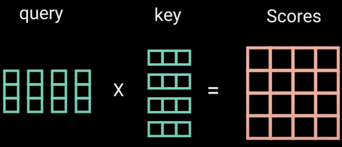
The query & key are multiplied to generate attention scores.
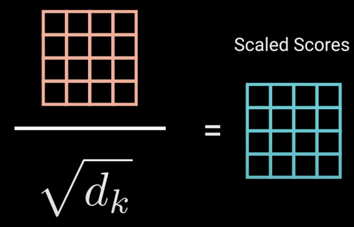
These are then scaled down by the square root of dimensionality to prevent holding softmax in its saturated regions and avoid vanishing gradients.
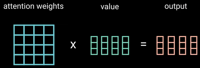
Finally, we multiply these weights with the values to produce an output layer, which is processed through a linear layer to generate a result.
In terms of computational complexity, self-attention layers are faster than recurrent layers when the sequence length n is smaller than the representation dimensionality d, which is most often the case.
As a direct result of this, combined with the increased amount of computation that can be parallelized by minimising sequential operations, transformers improve on the state of the art both in terms of performance and training cost.
Transformers have set the stage for massive jumps in performance for natural language and temporal models, and form the basis for advancements such as Open AI’s GPT models, Google’s BERT, and Google’s Switch Transformer.
Improving Language Understanding by Generative Pre-Training (GPT)
GPT is a language model based on transformers that achieved great success in its time by pre-training the model in an unsupervised way on a large corpus, and then fine tuning the model for different downstream tasks. This technique of performing task-agnostic training followed by fine tuning was distinguished from the training task-specific models, which had previously achieved state of the art performance.
Unsupervised Pre-Training
During pre-training, a neural network is used to maximize the likelihood of the next token given the previous k tokens. Concretely, given an unlabeled corpus U= {u₁, u₂, …, uₙ}, the likelihood L₁(U):
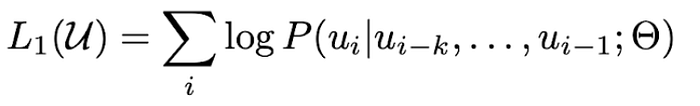
is maximized using stochastic gradient descent over the parameters 𝚯 of a transformer decoder (shown below), which models the conditional probability P.
Supervised Fine Tuning
Objective Functions
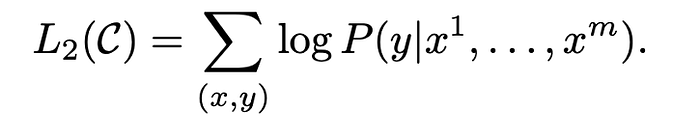
Once the transformer model has been pre-trained, a new linear (fully connected) layer is attached to the output of the transformer which is then passed through a softmax function to produce the output required for the specific task, such as Natural Language Inference, Question Answering, Document Similarity, and Classification. The model is fine tuned on each of these supervised tasks using labelled datasets. The the supervised objective function over a labelled dataset C with a data point: (x = (x₁,…,xₘ),y) then becomes L₂(C):
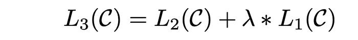
Sometimes to improve performance, language modeling objective (L₁(C)) is added to the fine-tuning objective with a regularization term to achieve the final loss L₃(C):
Input transformations
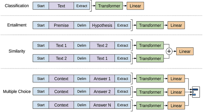
Common to all taks is the fact that the input is sandwiching the input text in between randomly initialized start and end tokens.
In Classification, the standard input transformation of using a start and end token around the input text is used.
In Natural language inference (Entailment), the premise and hypothesis are separated by the delimiter token ($).
In (Text) Similarity, two texts are separated by the delimiter token ($) and passed through the transformer once, and then a second time with the order of the texts swapped. Each output is then concatenated and passed through the linear+softmax layer. This is because there is no inherent order present in a similarity task.
In the Multiple Choice Question Answering task, the context, question, and each answer is separated with a delimiter ($) and passed through the transformer and linear layer independently. Finally, the linear output of each possible answer is passed through a softmax to get a normalized probability distribution over possible choices.
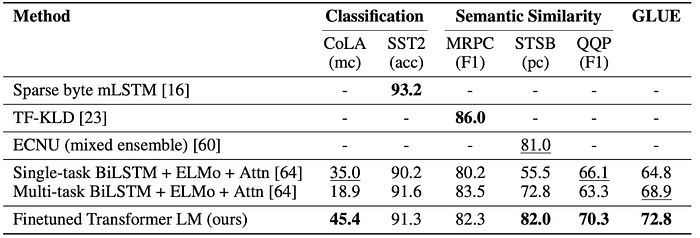
Performance of GPT
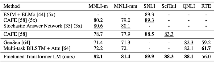
Natural Language Inference (NLI)
GPT outperformed state of the art models on all NLI datasets except Recognizing Textual Entailment (RTE).
Question Answering (QA)
GPT outperformed other state of the art models on all QA datasets.
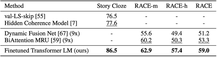
Similarity and Classification
GPT outperformed on most semantic similarity and classification datasets except the Stanford Sentiment Treebank (SST2) and Microsoft Research Paraphrase Corpus (MRPC).
BERT: Pre-training of Deep Bidirectional Transformers for Language Understanding
BERT is a product of Google AI, and a truly creative spin on transformers and the attention mechanism. Transformer models are directional, that is, they read the text input sequentially. BERT uses just the transformer encoder, along with bidirectional self-attention, which reads the entire sequence of words at once, in order to learn the context of a word based on the sequence succeeding & preceding it.
There are two BERT architectures: BERTBASE, with 110M parameters and 12 tranformer blocks, and BERTLARGE with 340M parameters and 24 transformer blocks. The implementation can be broken down into two steps: pre-training and fine tuning. These two steps allow for good performance using a smaller training corpus, since the pre-training step can use unlabelled data while relying on fine-tuning using labelled data to compensate for lost information.
Unsupervised Pre-training
Pre-training on BERT can be broken down into two tasks, and trains using a combined loss of both:
- Masked Language Model (MLM): 15% of the words in each input sequence are masked (replaced with a [MASK] token), and the model attempts to predict original value of each masked word.
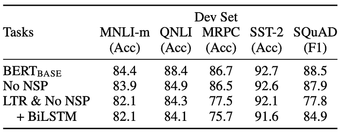
- Next Sentence Prediction (NSP): Data are input as sentence pairs, separated by a [SEP] token. 50% of pairs are randomized, 50% are in their original sequence. The model attempts to predict whether the second sentence IsNext or NotNext. The NSP component of the loss allows BERT to be more generalizable to tasks like Question Answering and Natural Language Inference.
Supervised Fine Tuning
Fine-tuning with BERT is straightforward. It uses labelled data, and for each language model task, we simply plug in the task specific inputs and labels into BERT and fine tune all the parameters.
Performance
BERT shows performance improvements over the state of the art for 11 natural language tasks, and drastically reduces training time for transfer-learning models by requiring only hyper-parameter tuning for many NLP tasks. It is the first fine-tuning based representation model that achieves state-of-the-art performance on a large suite of sentence-level and token-level tasks, outperforming many task-specific architectures.
The importance of its key innovation, bidirectional self-attention, is demonstrated in the ablation study below.
Switch Transformer: Scaling to Trillion Parameter Models with Simple and Efficient Sparsity
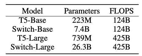
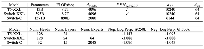
Switch Transformers introduced by researchers from Google appears to be the largest language model to be trained till date. Compared to the other large models like Open AI’s GPT-3, which has 175 Billion parameters, and Google’s T5-XXL, which has 13 Billion parameters, the largest Switch Model, Switch-C, has a whopping 1.571 Trillion parameters! This model was trained on the 807GB “Colossal Clean Crawled Corpus”(C4). Their efforts to increase model size are based on research that suggests models with simpler architectures but more parameters, data and computational budget perform better than more complicated models.
From Mixture of Experts (MoE) to the Switching Layer
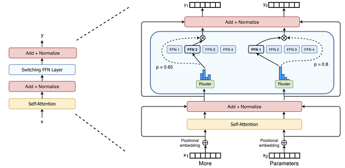
The switch transformer was able to achieve this parameter scale by using Mixture of Expert (MoE) models. Unlike traditional deep learning models, which use the same parameters for all inputs, MoE models use different parameters for each input. This results in a sparsely activated model, which can have many more parameters while maintaining the same computational budget as a model with parameters equal to those that are activated at any given time. For instance, a dense feed forward layer with N nodes can be transformed into a sparse MoE layer by having K dense feed forward layers with N nodes each and a trainable routing function to direct the input to one or more of them. The routing function is a vector of size N, Wᵣ, with trainable parameters which when multiplied with the input x, and normalized via softmax, produces a probability distribution over the N expert layers. For each expert i, we get pᵢ(x) = softmax(Wᵣ x)ᵢ.The output, y, of the MoE layer is the weighted sum of the outputs of the top-k experts. Concretely, if T is the set of top-k indices, and output from expert i ∈ T is Eᵢ(x), then y = ∑ᵢpᵢ(x)Eᵢ(x).
Creators of the switch transformer, Fedus, Zoph, et al., went against prevailing views by using only one expert (k=1) at each MoE routing layer to create the eponymous layer of the Switch Transformer. Earlier, researchers had intuited that at least two or more experts would be needed to learn how to route, and others reported that in models with many routing layers higher values of k in top-k routing were needed in layers closer to the input. However, the creators of the switch transformer go on to show that the switch-transformer can perform well on many NLU tasks, while saving computation and communication cost.
Using Model, Data, and Expert Parallelism
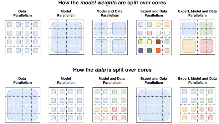
The switch transformer is able to scale up well because they are able to minimize communication requirements by using model, data, and expert parallelism. Their Switch-C model (1.5T parameters), uses data and expert parallelism, whereas the Switch-XXL (397B parameters), uses data, model, and expert parallelism.
Expert parallelism implies that weights of each expert lie in a different core. Thus when a batch B of inputs of size T reaches the router function, it must route each input to the right expert. To fix the maximum computation on any one expert, the maximum number of input tokens routed to each are also fixed. This number is called ‘expert capacity’. Expert capacity is the batch size of batch size of each expert calculated as (T/N) * capacity factor. If more tokens are routed to an expert than it’s capacity, i.e. when tokens overflow, they are passed onto the next layer through a residual connection. Scaling expert capacity using the capacity factor (a hyper parameter) helps mitigate token overflow.

Reducing Communication cost with Selective Precision
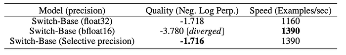
Another interesting problem solved by the authors of this work is using low precision numbers, such as ‘bfloat16’. ‘bfloat16’ is Google Brain’s 16 bit float precision format (b for brain) created by truncating float32 to the first 16 bits. In prior MoE works, using bfloat16 precision caused instability during training and forced the use of float32 precision. The creators of the switch transformer circumvented this issue by using high precision numbers only in the router computation, which is local to a given core, and showed that training still converges. This reduced the communication cost between cores by two, and increased throughput (speed).
Performance of the Switch Transformer
Fine Tuning Results
Switch models show performance improvement in all but one downstream fine tuning task: the AI2 Reasoning Challenge (ARC). Overall they saw gains with increasing model size, and also gains in both knowledge heavy and reasoning tasks, when compared to their FLOP matched baselines.

Scaling Properties
Scaling on the basis of training steps
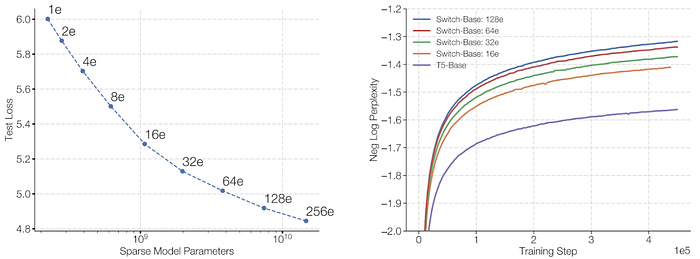
The authors found that more experts achieve lower loss and higher performance for a fixed number of steps, when the amount of computation (FLOPs) per token is held constant (left figure below). This means that sparser models learn faster in terms of number of training steps. Their switch-base 64 model achieved a 7.5x speed up in terms of step time compared to the T5-base model (not shown in the figure below). The plot on the right implies that larger models are more sample efficient, i.e, learn faster for a fixed number of observed samples.
Scaling on the basis of training time
The authors wished to understand that for a fixed training duration and computational budget, should one train a dense or a sparse model?
First, they noted that their sparse models outperformed the dense baselines: the model with 64 experts achieves a given loss 7x faster than T5-Base.
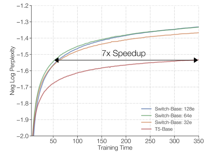
However, instead of comparing the sparse model with the same number of parameters, what if we compare a sparse model to a larger dense model? The following plot shows that the Switch-Base with 64 experts is more sample efficient (left) and 2.5x faster (right) than even T5-Large.
Diving deeper into time to train of the largest models, we see that the Switch-C model gets to a fixed perplexity (-1.096) four times faster than T5-XXL, while maintaing the same computational budget. Note the multiplier is four and not two because the reported value is in the logarithmic domain.
Note: Please refer to the paper for more interesting experiments and techniques that we haven’t discussed in this summary.
References
- Vaswani, et al. (2017). Attention Is All You Need. arXiv:1706.03762v5.
- Rashford, et. al. (2018) “Improving Language Understanding using Generative Pre-Training” https://cdn.openai.com/research-covers/language-unsupervised/language_understanding_paper.pdf
- Devlin, et al. (2019). BERT: Pre-training of Deep Bidirectional Transformers for Language Understanding. arXiv:1810.04805v2.
- Fedus, et al. (2021) “Switch Transformers: Scaling to Trillion Parameter Models using Simple and Efficient Sparsity” https://arxiv.org/pdf/2101.03961.pdf
- Graphics used from: https://www.youtube.com/watch?v=4Bdc55j80l8&t=300s&ab_channel=TheA.I.Hacker-MichaelPhi